Note

This article is from the BitPost 30 Day Challegne and was orignally posted there

A few days ago I wrote on article on Deep Neural Networks(DNN) in which I explained the mathematics behind a Perceptron, which is the most basic form of deep learning and the building block for more complex deep neural networks. In that article I promised to go into more detail on different kinds of neural networks and for the first one I wanted to cover Convolutional Neural Networks(CNN), this is mainly because it is used in the Computer Vision domain, which aims to use computers to obtain understanding from images and videos, this allows me to easily explain what the model is actual doing using visual representations.

A CNN is like a standard DNN in the fact that it has layers of neurons that are connect to each other and at each layer there is some mathematical operation taking place. With a standard neural network this is just a group of linear equations because each neuron is just multiplying the input by its weight value and adding a bias value (y = W*x + b were x is the input y is the output and W, b are the parameters of a neuron we are training). A CNN is different in that it needs to act on a 3-dimensional array of values instead of just a single value, this because of the way we represent images as data. Images cannot easily be understood by computers and we always need the input to our deep learning model to be a numeric representation of the data. To convert images to numeric values what we usually do is represent the red, blue and green intensity of each pixel on our display as a 2D array were the higher the value the more intense the color (with 8-bit color images this would be a value from 0 to 255) that are then stacked together into a 3D array (There can also be 4D arrays where a gamma value is added). Now that we have a 3D array we want to do some mathematical operation on it to produce meaningful information. The way a CNN does this is through the use of filters, a filter is a 2D array that is smaller than the image it is filtering and contains weights at each index of the array that can be trained (like the weight and bias value of the standard neuron). We use this filter by multiplying it against a subset of an image array that is the same size as the filter to obtain a new pixel value, we then move the filter over one pixel (or more if you want to compress the image) and do the same thing until we have produced a new image that hopefully maintains some important features (features could be anything the computer seems to think are important).

Here is a visual example.

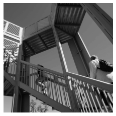
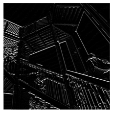
Say we want to find the edges of this image, a way to do this is to pass a very specific convolutional filter ([[-1,0,1], [-2,0,2], [-1,0,1]]) over the image. The reason this works is because of what we visually identify as an edge, they tend to have pretty high visual contrast between the sides the edge creates so this filter is a way of returning high pixel intensity values for the pixels with the highest contrast between their neighbors (this is just one way of doing edge detection). The output of this convolution is show below, here the input image way actually a 2D array since it was black and white so the output will also a 2D array again show in black and white.

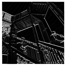
Another important idea in CNNs is the use of pooling, which is when we reduce the total number of pixels in the image while trying to retain the features highlighted during the convolution. We can also reduce the size of the output image during the convolutional filtering by increasing something called the stride, the number of pixels the filter is moved at each step, if we increase the stride the total number of pixels will be less. Pooling is different in that we are using some mathematical operation to combine blocks of pixels into a single pixel, this could be either taking the average of the pixels or only using the highest value, it all depends on the application it is being used in. For the example we have been using we want to increase the contrast on the edges as much as possible so to do this we can use a max pooling operation, which uses the max value from the block of pixels as the new pixel value. If we do this on 2 by 2 sections of the image this is the result.

So far we have talked about what a convolution is but I haven't yet explained how this is actually used for machine learning. Typically convolutional layers are not used by themselves, we still need a traditional DNN connected to our convolutional layers to make predictions, so the convolutional layers are more of a tool for extracting important information from the images (features) for the DNN to use. There are many different applications where you could use CNNs to do a task but I think the most common ones are object detection and image prediction. Object detection is identifying one or more objects in an image (including their location) while image predication is saying whether or not an image represents some class (cat/dog/pig/llama, pizza/not pizza, etc.), they do this by training on a dataset of images that have labels associated with them so that after the image has passed through the convolutional layers it is sent to a layer (can also be more than one) of standard neurons that then produce a prediction on the class of the image or the location of an object. We can then use the standard back propagation gradient descent algorithm I discussed in the Deep Neural Networks article to train the model, which will also train the convolutional filter weights.

To give you an example I have made a quick model using a python library/framework called TensorFlow, the model will predict whether or not an image contains a dog or a cat (it assumes that one of the two will be present). Here is the model architecture :

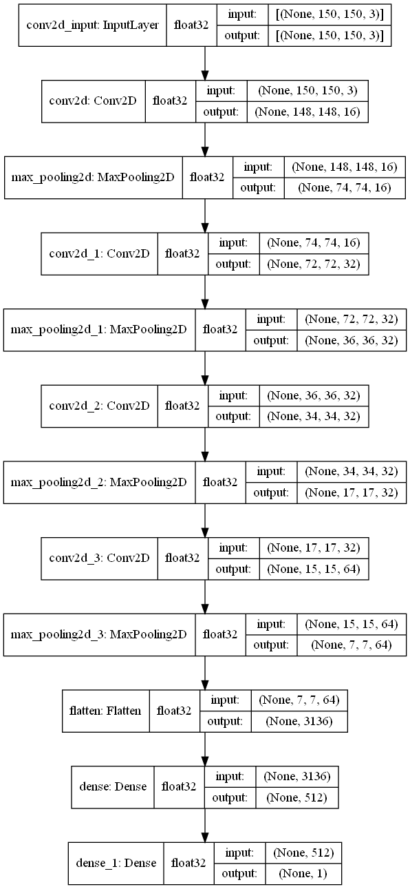
This image shows the shape of the input and output of each layer in the model and I want to walk through these. The first layer is just an input which accepts 150 by 150 RGB encoded images (a 3D array), the next is a convolutional layer that takes in the image and applies 16 different filters to the image to produce a 3D array with depth 16. We then have a max pooling layer which reduces the number of pixels in each of the 16 2D arrays by half (using the max of the pixel blocks like discussed earlier). Then we have 3 more sets of a convolution layer followed by a max pooling layer, the first two convolutions will have 32 filters and the last one will have 64 filters. Then we flatten the output of the last max pooling layer so that we can feed it into the DNN, which only has two layers. The first is the hidden layer that will provided the prediction functionality, and the last is the output layer that tells use whether the image is of a cat or a dog. To see how the model is functioning, after I trained it I gave it the image of a dog shown below and wrote a script that would display the outputs from a specific convolution or max pooling layer.

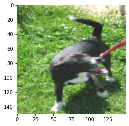
Here are some of the more interesting images produced after the first set of convolution and max pooling layers.

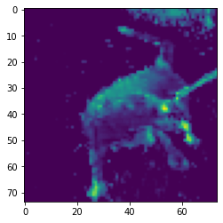
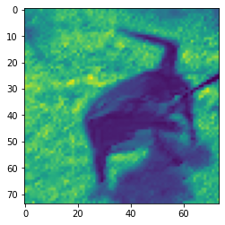
As you can see these are not quite as clear as the edge detection example, but this is to be expected. The computer is not trying to identify edges but instead trying to identify features it thinks are important for determining whether an image is of a cat or a dog and images are probably not the most important feature for that task.

Thanks for reading

Zach

PS Here is the code the recreate the model I used for this article and plot the outputs from each of the convolution or max pooling layers.

First download some data.

curl https://storage.googleapis.com/mledu-datasets/cats_and_dogs_filtered.zip -O cats_and_dogs_filtered.zip

import os
import zipfile
import tensorflow as tf
import numpy as np
mport matplotlib.pyplot as plt
import matplotlib.image as mpimg

from PIL import Image
from tensorflow.keras.preprocessing.image import ImageDataGenerator 
from tensorflow.keras.optimizers import RMSprop

#Unzip file and save to /data subdirectory
local_zip = 'cats_and_dogs_filtered.zip'
zip_ref = zipfile.ZipFile(local_zip, 'r')
zip_ref.extractall('./data')
zip_ref.close()

base_dir = './data/cats_and_dogs_filtered'
train_dir = os.path.join(base_dir, 'train')
val_dir = os.path.join(base_dir, 'validation')

train_cat_dir = os.path.join(train_dir, 'cats')
train_dog_dir = os.path.join(train_dir, 'dogs')

val_cat_dir = os.path.join(val_dir, 'cats')
val_dog_dir = os.path.join(val_dir, 'dogs')


train_cat_len = len(os.listdir(train_cat_dir))
train_dog_len = len(os.listdir(train_dog_dir))

val_cat_len = len(os.listdir(val_cat_dir))
val_dog_len = len(os.listdir(val_dog_dir))

print(f'There are {train_cat_len + train_dog_len} training files, \n{train_cat_len} are cats, {train_dog_len} are dogs')
print(f'There are {val_cat_len + val_dog_len} training files, \n{val_cat_len} are cats, {val_dog_len} are dogs')

model = tf.keras.models.Sequential([
    tf.keras.layers.Conv2D(16, (3, 3), activation='relu', input_shape=(150, 150, 3)),
    tf.keras.layers.MaxPool2D(2, 2),
    tf.keras.layers.Conv2D(32, (3, 3), activation='relu'),
    tf.keras.layers.MaxPool2D(2, 2),
    tf.keras.layers.Conv2D(32, (3, 3), activation='relu'),
    tf.keras.layers.MaxPool2D(2, 2),
    tf.keras.layers.Conv2D(64, (3, 3), activation='relu'),
    tf.keras.layers.MaxPool2D(2, 2), 
    tf.keras.layers.Flatten(),
    tf.keras.layers.Dense(512, activation='relu'),
    tf.keras.layers.Dense(1, activation='sigmoid')
])

model.summary()

# Uncomment to save image of model
# tf.keras.utils.plot_model(model, to_file='dog_or_cat.png', show_shapes=True, show_dtype=True, show_layer_names=True)

model.compile(
    optimizer=RMSprop(learning_rate=0.001),
    loss='binary_crossentropy',
    metrics=['accuracy']
 )

train_datagen = ImageDataGenerator(rescale=1.0/255.0)
train_generator = train_datagen.flow_from_directory(
    train_dir,
    target_size=(150, 150),
    batch_size=128,
    class_mode='binary'
)
val_generator = train_datagen.flow_from_directory(
    val_dir,
    target_size=(150, 150),
    batch_size=80,
    class_mode='binary'
)

history = model.fit(
    train_generator,
    validation_data = val_generator,
    epochs = 10,
    steps_per_epoch=8,
    validation_steps=8
)


# Change index of output_layer to see the output from different convolution layers
input_layer = history.model.layers[0]
print(f'Using input layer {input_layer.name}')
output_layer = history.model.layers[3]
print(f'Using output layer {output_layer.name}')

  

first_convolution_layer_function = tf.keras.backend.function(
    [input_layer.input], 
    [output_layer.output]
)

  

img = Image.open('./path/to/image')
img = img.resize((150, 150))
img = np.array(img)
plt.imshow(img)
plt.show()

first_convolution_layer_output = first_convolution_layer_function(tf.constant([img]))
img_array = first_convolution_layer_output[0][0, :, :, :]
for i in range(img_array.shape[-1]):
    flat = img_array[:, :, i]
    plt.imshow(flat)
    plt.show()